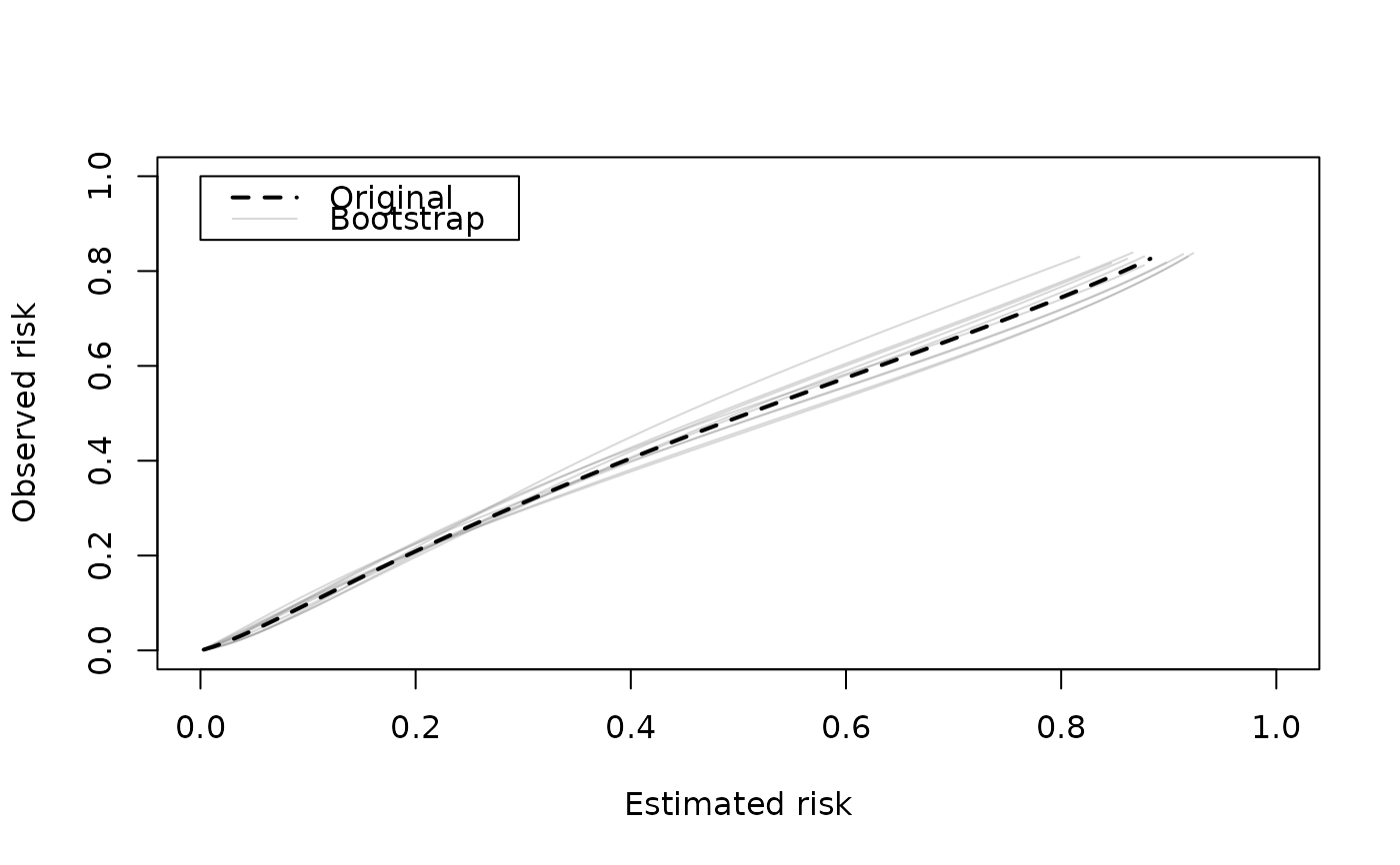
Plot calibration stability across bootstrap replicates — calibration

A calibration (in)stability plot shows calibration curves for bootstrap models evaluated on original outcome. A stable model should produce boot calibration curves that differ minimally from the 'apparent' curve. See Riley and Collins (2023).

Usage

calibration_stability(x, calib_args, xlim, ylim, xlab, ylab, col)

Arguments

x: an object produced by validate with method = "boot_\*" (or boot_optimism with method="boot")
calib_args: settings for calibration curve (see pmcalibration::pmcalibration). If unspecified settings are given by cal_defaults with 'eval' set to 100 (evaluate each curve at 100 points between min and max prediction).
xlim: x limits (default = c(0,1))
ylim: y limits (default = c(0,1))
xlab: a title for the x axis
ylab: a title for the y axis
col: color of lines for bootstrap models (default = grDevices::grey(.5, .3))

Value

plots calibration (in)stability. Invisibly returns a list containing data for each curve (p=x-axis, pc=y-axis). The first element of this list is the apparent curve (original model on original outcome).

References

Riley RD, Collins GS. (2023). Stability of clinical prediction models developed using statistical or machine learning methods. Biom J. doi:10.1002/bimj.202200302. Epub ahead of print.

Examples

set.seed(456)
# simulate data with two predictors that interact
dat <- pmcalibration::sim_dat(N = 2000, a1 = -2, a3 = -.3)
mean(dat$y)
#> [1] 0.1985
dat$LP <- NULL # remove linear predictor

# fit a (misspecified) logistic regression model
m1 <- glm(y ~ ., data=dat, family="binomial")

# internal validation of m1 via bootstrap optimism with 10 resamples
# B = 10 for example but should be >= 200 in practice
m1_iv <- validate(m1, method="boot_optimism", B=10)
#> It is recommended that B >= 200 for bootstrap validation

calibration_stability(m1_iv)